DE/python
시계열 시뮬레이션 | 실전시계열 분석 4장
주홍철(최고의 개발자), you(C++ 마스터)2023.12.07
용어 : 박스-젠킨스 모델(Box-Jenkins Model)
박스-젠킨스 모델(Box-Jenkins Model)은 시계열 데이터 분석에 사용되는 통계적 방법론
이 모델의 핵심은 ARIMA(Autoregressive Integrated Moving Average) 모델
ARIMA 모델은 세 가지 주요 구성요소로 이루어져 있다.
- 자기회귀(AR: Autoregressive): 과거는 미래를 예측한다.

- 차분(I: Integrated) : 비정상성을 제거하기 위해 각 시점에서 이전 시점의 값을 뺍니다. Yt = Yt - Y(t-1) 입니다. 차분은 시계열 데이터의 추세나 계절성과 같은 비정상적인 요소를 제거하여 ARIMA 모델이 데이터의 순수한 자기상관성에만 집중할 수 있게 도와줍니다.
- 이동 평균(MA: Moving Average): 예측 오차들의 평균을 이용해서 현재값을 설명합니다.
용어 : 사전관찰
어떻게든 미래에 일어날 일에 대한 정보가 모델에서 시간을 거슬러 전파되어 모델의 초기 동작에 영향을 주는 방법입니다.
용어 : 포워드 필
누락된 값이 나타나기 직전의 값으로 누락된 값을 채우는 가장 간단한 방법
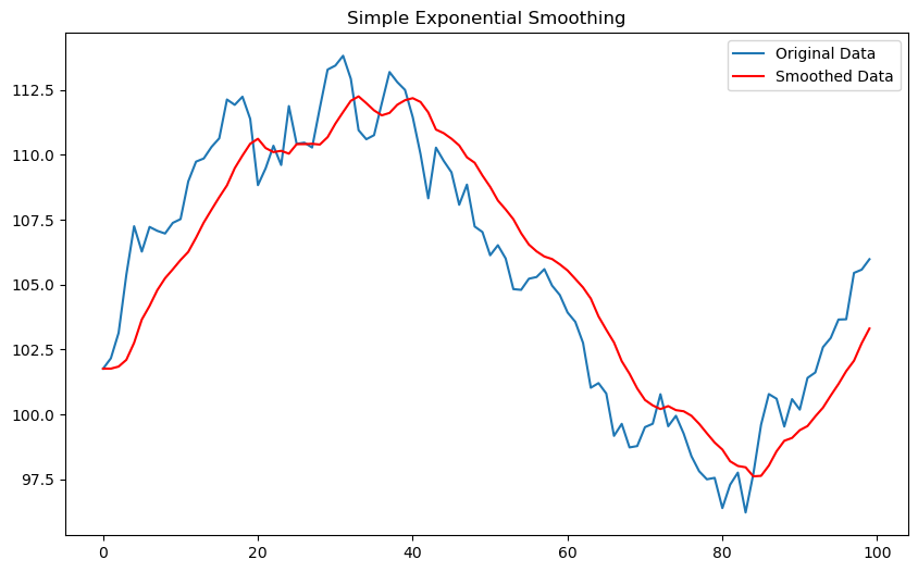
용어 : 지수평활
최근데이터에 더 높은 가중치를 부여하는 방법. 시계열 데이터의 최근 관측값이 미래값을 예측하는데 더 중요하다는 근거하에 쓰는 기법. 3가지의 기법이 존재 합니다.
지수이동평균(EMA)과의 차이점은 지수평활은 시계열 데이터의 특성에 따라 다양한 방식으로 가중치를 적용할 수 있습니다. 예를 들어, 단순 지수평활은 일정한 가중치를 적용하지만, 홀트-윈터스 방법은 추세와 계절성에 따라 다르게 가중치를 적용합니다.
- 단순 지수평활(Simple Exponential Smoothing): 추세, 계절성 없을 때 사용, 지수적으로 감소하는 과거부터 가중치 적용
- 홀트(Holt)의 선형 추세 방법: 추세있을 때 사용
- 홀트-윈터스(Holt-Winters) 방법: 계절성이 있을 때 활용
코드
import numpy as np
import pandas as pd
from statsmodels.tsa.api import SimpleExpSmoothing
import matplotlib.pyplot as plt

# 임의의 시계열 데이터 생성
np.random.seed(0)
data = np.random.randn(100).cumsum() + 100  # 누적합리스트 생성

# numpy to pandas
data_series = pd.Series(data)

# 단순 지수평활 모델 생성
model = SimpleExpSmoothing(data_series)
model_fit = model.fit(smoothing_level=0.2)

# 예측 결과
fitted_values = model_fit.fittedvalues

# 원본 데이터와 예측 결과 시각화
plt.figure(figsize=(10,6))
plt.plot(data_series, label='Original Data')
plt.plot(fitted_values, label='Smoothed Data', color='red')
plt.title('Simple Exponential Smoothing')
plt.legend()
plt.show()
택시 TS 시뮬레이션
import numpy as np
from dataclasses import dataclass
import matplotlib.pyplot as plt
import seaborn as sns
import queue
from collections import defaultdict
@dataclass
class TimePoint:
taxi_id: int
name: str
time: float
def __lt__(self, other):
return self.time < other.time
def taxi_id_number(num_taxis):
arr = np.arange(num_taxis)
np.random.shuffle(arr)
for i in range(num_taxis):
yield arr[i]
def shift_info():
start_times_and_freqs = [(0, 8), (8, 30), (16, 15)]
indices = np.arange(len(start_times_and_freqs))
while True:
idx = np.random.choice(indices, p=[0.25, 0.5, 0.25])
start = start_times_and_freqs[idx]
yield (start[0], start[0] + 7.5, start[1])
def taxi_process(taxi_id_generator, shift_info_generator):
taxi_id = next(taxi_id_generator)
shift_start, shift_end, shift_mean_trips = next(shift_info_generator)
actual_trips = round(np.random.normal(loc=shift_mean_trips, scale=2))
average_trip_time = 6.5 / shift_mean_trips * 60
between_events_time = 1.0 / (shift_mean_trips - 1) * 60
time = shift_start
yield TimePoint(taxi_id, 'start shift', time)
deltaT = np.random.poisson(between_events_time) / 60
time += deltaT
for i in range(actual_trips):
yield TimePoint(taxi_id, 'pick up', time)
deltaT = np.random.poisson(average_trip_time) / 60
time += deltaT
yield TimePoint(taxi_id, 'drop off', time)
deltaT = np.random.poisson(between_events_time) / 60
time += deltaT
deltaT = np.random.poisson(between_events_time) / 60
time += deltaT
yield TimePoint(taxi_id, 'end shift', time)
class Simulator:
def __init__(self, num_taxis):
self._time_points = queue.PriorityQueue()
taxi_id_generator = taxi_id_number(num_taxis)
shift_info_generator = shift_info()
self._taxis = [taxi_process(taxi_id_generator, shift_info_generator) for i in range(num_taxis)]
self._prepare_run()
def _prepare_run(self):
for t in self._taxis:
while True:
try:
e = next(t)
self._time_points.put(e)
except StopIteration:
break
def run(self):
sim_data = defaultdict(list)
sim_time = 0
while sim_time < 24:
if self._time_points.empty():
break
p = self._time_points.get()
sim_time = p.time
sim_data[p.taxi_id].append((p.time, p.name))
return sim_data
# 시뮬레이션 실행
sim = Simulator(1000)
data = sim.run()
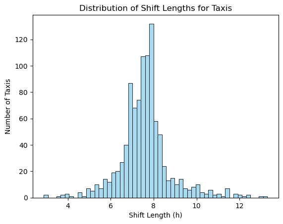
# 택시 별 근무 시간 분포
shift_lengths = [activities[-1][0] - activities[0][0] for activities in data.values()]
sns.histplot(shift_lengths, kde=False, color='skyblue')
plt.xlabel('Shift Length (h)')
plt.ylabel('Number of Taxis')
plt.title('Distribution of Shift Lengths for Taxis')
plt.show()
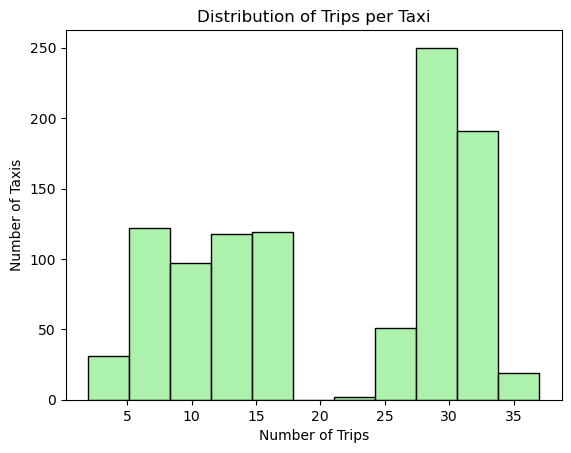
# 3. 운행 횟수 분포 (개선된 색상)
sns.histplot(trip_counts, kde=False, color='lightgreen')
plt.xlabel('Number of Trips')
plt.ylabel('Number of Taxis')
plt.title('Distribution of Trips per Taxi')
plt.show()
# 첫 5대 택시의 데이터를 선택
first_five_taxis_data = {taxi_id: data[taxi_id] for taxi_id in list(data)[:1]}
# 선택된 데이터 출력
for taxi_id, activities in first_five_taxis_data.items():
print(f"Taxi ID: {taxi_id}")
for time, activity in activities:
print(f" Time: {time}, Activity: {activity}")
print()
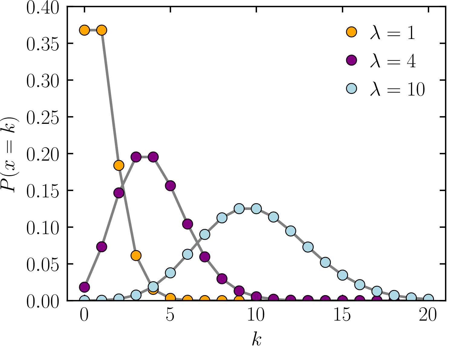
포아송 분포
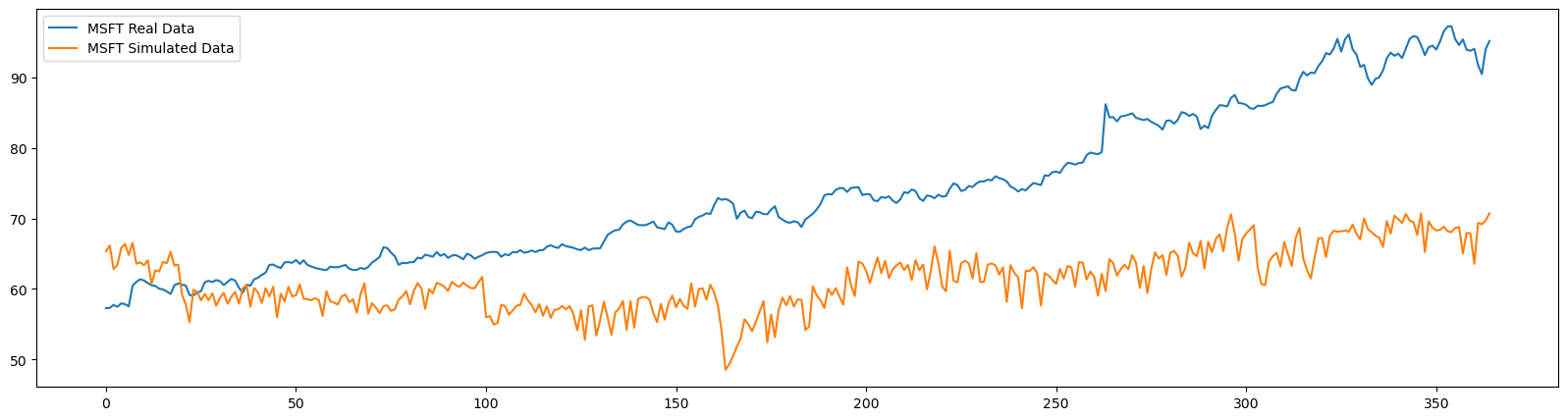
오토인코더를 통한 주식 차트 시뮬레이션
오토인코더 네트워크는 실제로 인코더와 디코더라는 두 개의 연결된 네트워크 쌍

기존 오토인코더의 문제점은 벡터 보간이 용이하지 않을 수 있음.ex) mnist에서 1과 7의 차이 / 오토인코더는 다음과 같은 큰 특징이 있음.
변분 오토인코더(Variational Autoencoder, VAE)
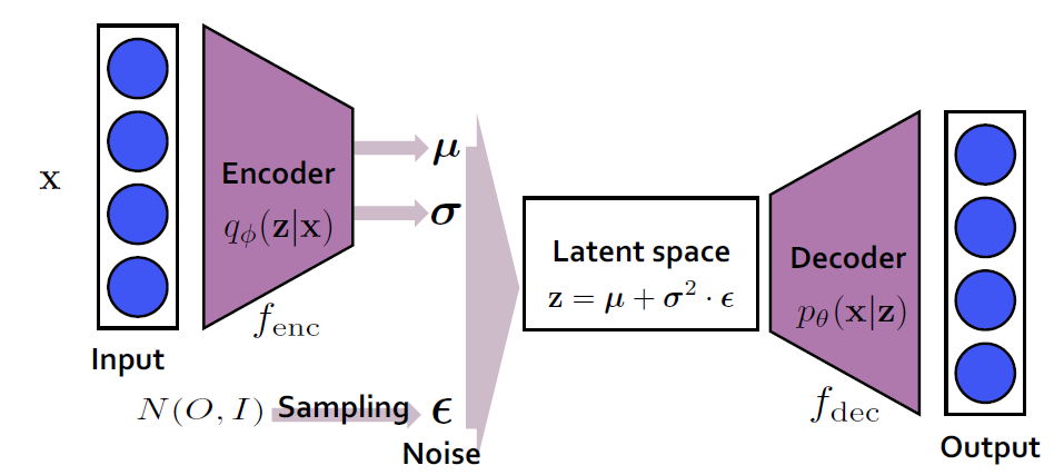
여기서 나온 것이 바로 변분 오토인코더(Variational Autoencoder, VAE)임. 이는 딥러닝과 확률론을 결합한 생성적 모델 중 하나.
다음과 같은 구조를 가짐.
- 인코더
- 리파라미터화 트릭 - 리파라미터화 트릭(Reparameterization Trick)
- 디코더
import yfinance as yf
import torch
import torch.nn as nn
import torch.optim as optim
from torch.utils.data import DataLoader, TensorDataset
import numpy as np
import matplotlib.pyplot as plt
from sklearn import preprocessing
import quandl
quandl_data_apple = quandl.get("WIKI/AAPL")
quandl_data_amazon = quandl.get("WIKI/AMZN")
quandl_data_msft = quandl.get("WIKI/MSFT")
# 1980 ~ 2018 까지의 데이터 : 고가 중심으로.
msft_high_raw = (quandl_data_msft['High'].values).reshape(1,-1)
msft_high = preprocessing.normalize(msft_high_raw, norm='max', axis=1)
msft_high = msft_high.reshape(msft_high.shape[1],)
msft_max_high = np.max(msft_high_raw)

apple_high_raw = (quandl_data_apple['High'].values).reshape(1,-1)
apple_high = preprocessing.normalize(apple_high_raw, norm='max', axis=1)
apple_high = apple_high.reshape(apple_high.shape[1],)
apple_max_high = np.max(apple_high_raw)

amazon_high_raw = (quandl_data_amazon['High'].values).reshape(1,-1)
amazon_high = preprocessing.normalize(amazon_high_raw, norm='max', axis=1)
amazon_high = amazon_high.reshape(amazon_high.shape[1],)
amazon_max_high = np.max(amazon_high_raw)

# Generate samples
def generate_samples(data, sample_size):
    n_samples = data.shape[0] // sample_size
    return np.array([data[i*sample_size:(i+1)*sample_size] for i in range(n_samples)])

test_data_points = 365
sample_size = 365

def split_data(high):
    return high[:-test_data_points], high[-test_data_points:]

msft_high_train, msft_high_test = split_data(msft_high)
X_msft_train = generate_samples(msft_high_train, sample_size)
X_msft_test = generate_samples(msft_high_test, sample_size)

X_msft_train_tensor = torch.tensor(X_msft_train, dtype=torch.float32)
X_msft_test_tensor = torch.tensor(X_msft_test, dtype=torch.float32)

class VAE(nn.Module):
    def __init__(self, input_size, latent_dim):
        super(VAE, self).__init__()
        # Encoder
        self.fc1 = nn.Linear(input_size, 256)
        self.fc21 = nn.Linear(256, latent_dim)
        self.fc22 = nn.Linear(256, latent_dim)
        # Decoder
        self.fc3 = nn.Linear(latent_dim, 256)
        self.fc4 = nn.Linear(256, input_size)

    def encode(self, x):
        h1 = F.relu(self.fc1(x))
        return self.fc21(h1), self.fc22(h1)

    def reparameterize(self, mu, logvar):
        std = torch.exp(0.5 * logvar)
        eps = torch.randn_like(std)
        return mu + eps * std

    def decode(self, z):
        h3 = F.relu(self.fc3(z))
        return torch.tanh(self.fc4(h3))

    def forward(self, x):
        mu, logvar = self.encode(x)
        z = self.reparameterize(mu, logvar)
        return self.decode(z), mu, logvar

def loss_function(recon_x, x, mu, logvar):
    BCE = F.mse_loss(recon_x, x.view(-1, sample_size))
    KLD = -0.5 * torch.sum(1 + logvar - mu.pow(2) - logvar.exp())
    return BCE + KLD

model = VAE(sample_size, latent_dim=1)
optimizer = optim.Adam(model.parameters(), lr=0.01)
train_loader = DataLoader(TensorDataset(X_msft_train_tensor), batch_size=32, shuffle=True)

epochs = 300
for epoch in range(epochs):
    model.train()
    train_loss = 0
    for batch_idx, (data,) in enumerate(train_loader):
        optimizer.zero_grad()
        recon_batch, mu, logvar = model(data)
        loss = loss_function(recon_batch, data, mu, logvar)
        loss.backward()
        train_loss += loss.item()
        optimizer.step()

model.eval()
with torch.no_grad():
    msft_simulated_high = model(X_msft_test_tensor)[0].numpy()
참고자료
- http://vision-explorer.reactive.ai/#/galaxy?_k=12fku3
- https://www.youtube.com/watch?v=o_peo6U7IRM&t=375s
- https://towardsdatascience.com/intuitively-understanding-variational-autoencoders-1bfe67eb5daf
- https://medium.com/@ricardo.vrgl/generating-simulated-stock-price-data-using-a-variational-autoencoder-d18fc79fc623